Python算法代写 数据测试代写 算法代写 Python代写
923Python2 Python算法代写 测试数据 工单数量自由设定,先设定为 20 机器数量自由设定,先设定为 6,编号为[1 2 3 4 5 6] 工人数量自由设定,先设定为 2,编号为[1 2] PTq[5 10 15 20 25 5 10 15 20 25 5 10 15 20 2...
View detailsSearch the whole station
数值分析课业代写 Problem 1. Program the power method and inverse power method to compute the maximum and minimum eigenvalue/eigenvector pairs of the symmetric
Program the power method and inverse power method to compute the maximum and minimum eigenvalue/eigenvector pairs of the symmetric matrix A ∈ Rn×n.
To test your code, you can create a random eigenvalue decomposition with specified eigenvalues as follows:
Q = np.random.randn(n, n) # sample a matrix with iid N(0, 1) entries
Q = np.linalg.qr(Q)[0] # the Q factor in its QR decomposition is an
                       # orthogonal matrix sampled uniformly from
                       # the orthgonal group O(n)
Lam = np.diag(...) # set the diagonal matrix of eigenvalues manually
A = Q@Lam@Q.T # compute A from Q and Lam
This way you can fix the values of λ1 and λ2 (or 1/λn and 1/λn−1) to control the convergence rate of the (inverse) power method.
Make a plot (or several plots) of the convergence of the (inverse) power method for several different eigenvalue ratios. Since you set the eigenvalues of your test matrix A yourself, you can easily compare with the true solution. Your plot(s) should show evidence that the convergence rate is largely controlled by, e.g., λ2/λ1.
(Note: in this problem, I would like you to look at both the power method and the inverse power method. For the inverse power method, use np.linalg.lu or scipy.linalg.lu instead of your own LU decomposition to compute the LU decomposition of A. You can then use the function scipy.linalg.solve triangular to do the forward and backward solves involving your triangular factors.)
Incorporate shifts into your power method (i.e., apply the power method and inverse power method to the shifted matrix A − λI). Come up with a strategy for choosing the shift λ to accelerate the convergence of the power method. Note: the shift can vary from iteration to iteration. In general, there can be many possible strategies—you must simply come up with some strategy that reduces the overall number of iterations. However, be careful with the inverse power method: if you change the shift, you must recompute the LU decomposition used to apply (A − λI)−1 at each step.
Read about the compressed sparse row (CSR) sparse matrix format. SciPy provides a class implementing a sparse matrix using the CSR format: see scipy.sparse.csr matrix.
Set up a version of A for N = 64 using scipy.sparse.csr matrix. Next, read the documentation for the function scipy.sparse.linalg.eigsh. Use it to compute the k = 16 smallest nonzero eigenvalues and eigenvectors of A (hint: use the sigma keyword argument).
Using plt.subplot, make a 4 × 4 grid of 2D plots of each of the eigenvectors, as well as a plot of the eigenvalues that you compute.
a.
The matrix A can be interpreted as a graph. Its rows and columns are naturally identified with the nodes in the original lattice, which we think of as the graph’s vertices. There is an edge between a pair of vertices if the corresponding pair of nodes is adjacent in the lattice. Recall from lecture that A is a discretized Laplacian.
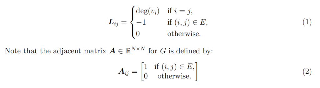
On the other hand, if we start with a graph G = (V, E), where N = |V | and V = {v1, . . . , vN} is the set of vertices and E = {(i, j) : viand vjare adjacent} is the set of edges, we can define the graph Laplacian L ∈ RN×N by:
Download a graph from:
https://sites.google.com/site/xiaomengsite/research/resources/graph-dataset
or some other website online. Load it using Python and build a CSR version of L for your graph. Next, as in Problem 3, use scipy.sparse.linalg.eigsh (note that L should be symmetric!) to compute the first k = 2 smallest nonzero eigenvalue and eigenvector pairs of L. Let u1 and u2 be these eigenvectors, and experiment with making plots of u1 and u2 to visualize the graph. Please be creative and feel free to experiment.
(Hint: the process of getting your graph into Python and building L may be annoying and require some data processing. Don’t be a hero—use a relatively simple graph to make this easy. Between a few hundred vertices and a few thousand vertices is a good target.)
b (bonus).
Compute u3 and make a 3D visualization of your graph. I recommend starting with mplot3d for 3D plotting, but feel free to contact me for more recommendations, and feel free to experiment.
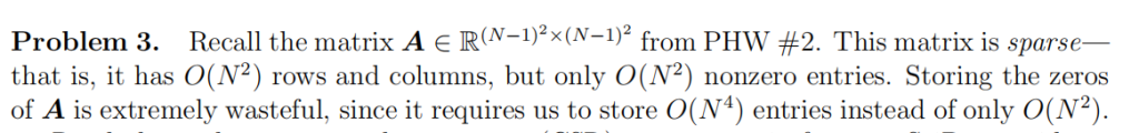
Read about bipartite graphs online. An off-diagonal block of the adjaceny matrix (not the graph Laplacian matrix L!) of your graph from Problem 4 is a bipartite graph. Pick such an off-diagonal block and denote it AI,J, where I and J are the row and column indices of the block (I ∩ J = ∅).
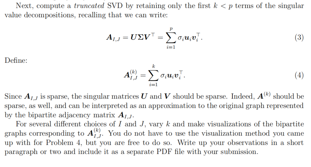
Let m = |I| and n = |J| and p = min(m, n). Compute the singular value decomposition AI,J= UΣV T, where U ∈ Rm×p, V ∈ Rn×p, and Σ ∈ Rp×p. Do this using np.linalg.svd with full matrices=False. Make a semilogy plot of the singular values σ1, . . . , σpand observe how rapidly they decay.

更多代写:C#代码代写 槍手代考英文 英国物理Final exam 温哥华essay代写 温哥华商务英文论文写作 留学speech代写
合作平台:essay代写 论文代写 写手招聘 英国留学生代写

Python2 Python算法代写 测试数据 工单数量自由设定,先设定为 20 机器数量自由设定,先设定为 6,编号为[1 2 3 4 5 6] 工人数量自由设定,先设定为 2,编号为[1 2] PTq[5 10 15 20 25 5 10 15 20 25 5 10 15 20 2...
View details
CS579/ECE599 Assignment Homework 1 物理攻击与对策代写 Please complete this assignment (100 pts total) and submit your report/program code on Canvas (all files compressed in one .zip witho...
View details
python code代写会不会是直接抄袭的其他源代码?怎么检验? python code代写 计算机程序的学习非常有用,能够做很多的工作,比如软件工程师、网络安全工程师等,国外的计算机行业也非常发达,去国外高校深造...
View details
Homework 2 FE621 Computational Methods in Finance 金融计算方法代写 For all the problems in this assignment you need to write computer programs an For all the problems in this assignment you ...
View details