实证金融作业代写 FNCE 435代写 Empirical Finance代写

FNCE 435 – Empirical Finance

Individual Assignment (Section I)

实证金融作业代写 (Important: This assignment is to be implemented on an individual basis. No sharing of material— including data, results, inferences and write-ups

(Important: This assignment is to be implemented on an individual basis. No sharing of material— including data, results, inferences and write-ups—may take place among members of a group nor across different groups.)

(About the significance level: For all the tests of significance in this assignment, please assume a 5% significance level.)

Examining Initiation of Dividend Payments

Dividend is a big thing in Finance. Much of shareholders’ return comes in the form of dividend payments. Yet, firms are not obligated to pay dividends. Being a choice of the firm, it is important to understand the implications of the firm’s decision on whether to pay or not to pay dividends.

In this assignment we will examine instances where firms start paying dividends. 实证金融作业代写

We base our analysis on a sample of firms that announce the initiation of dividend payments. Each datapoint consists of a firm and the date it announced that it would start paying dividends. (and the condition that the firm had not paid any dividends in the 10 years prior to that announcement). For each data point of our study—that is, for each firm and the date when it announced that it would start paying dividends—we also include another firm that did not announce initiation of dividends on that date. Data on dividend initiations and matched firms appear in the dataset “d_div.sas7bdat” (available on Canvas).

Figure 1 illustrates the sample by showing the first few observations in the dataset.

For each observation, the column INIT identifies whether it refers to a firm that initiates dividend (INIT=1) or does not initiate dividend (INIT=0). Take the first record. It says that the firm with PERMNO=13936 (“PHILLIPS VAN HEUSEN CORP”) declared in DCLRDT=April 8^th, 1970 that it was going to start paying dividends. The next row, with INIT=0, has the identification of a matched firm. More specifically, the firm with PERMNO=28265 (“UNITED FINANCIAL CORP CA”) had not paid any dividends in the 10-year period prior to April 8^th, 1970, and kept on not paying dividend in that date.

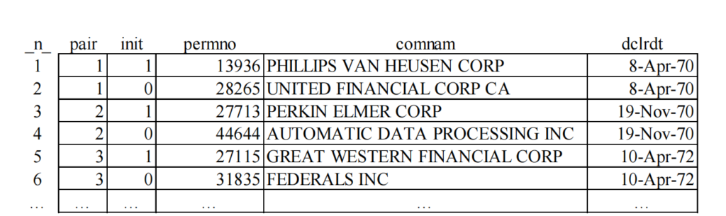
Figure 1. Example of data on dividend announcements

Why are we examining dividends? The baseline theory in Finance is that dividends do not matter: whether you return your money to shareholders via dividends or capital gains is irrelevant. On the other hand, people know that it is bad news when a firm decides to stop paying dividends (see Figures 4.4 and 4.5, module 4). Which suggests that dividends have valuation implications for the firm. We complement the analysis in module 4 by looking at situations when firm start (rather than quit) paying dividends.

There are at least three relevant questions that can be examined with respect to dividend initiations:

I. Do dividends have valuation implications? If so, markets should react to the firm’s decision to  start paying dividends. If dividends convey good news about the firm, market reactions should be positive.

II. What are the determinants of market reactions to the firm’s announcement that dividends will start being paid. In part I, one examines if markets react to the announcements. While here you examine in a regression framework what are the determinants of the market reactions to such announcements.

III. What characteristics seem to drive the firm’s decision to start paying dividends?

Part I: Valuation Implications 实证金融作业代写

We start our investigation by answering question (I):

Do dividends have valuation implications? If so, markets should react to the firm’s decision to start paying dividends. If dividends convey good news about the firm, market reactions should be positive.

You will address this question with an event study—employing the technique covered in module 4. For the sample of firms that announced the initiation of dividend payments, you will examine. And show the pattern of abnormal and cumulative abnormal returns over the 11-day window around the announcement day.

For the definition of abnormal return, use the constant-mean return model—that is, define abnormal return as the stock raw return (the variable RET in the CRSP dataset “dsf.sas7bdat”, located in “/wrds/crsp/sasdata/a_stock”) minus the average return of the company’s stock. For an announcement by company i at time t, define average return as the average of the variable RET for company i over the window [t – 365, t – 20]—that is, from 365 calendar days before the announcement date up to 20 calendar days before the announcement date. Important: notice that the abnormal return here is different from the abnormal return used in module 4. In module 4 we employed the market-adjusted return model while here we use the constant-mean return model.

Please examine formally whether markets react positively to dividend initiations. 实证金融作业代写

Prepare and show a table showing average abnormal returns, t-stats and p-value for 11-day window around announcements. Also create and show a graph with the pattern of average cumulative abnormal returns over the same 11-day window. Anchor your inferences on formal hypotheses testing. Also, examine whether markets respond efficiently to news in dividend initiations. (for this you can assume that some dividend announcements happen after the close of the market—that is, market reactions to such announcements could happen up to one day after the event date).

(Hint: notice that the examination here is based on 551 events—the observations in the dataset for which INIT=1.)

One criticism of the event study is that it might be capturing something else that happens around the announcement day. Let’s say, perhaps some other news that happen to be released together with announcements of dividend initiations affect many firms out there— including the ones announcing dividend initiations.

The use of abnormal returns aims at addressing this possibility. 实证金融作业代写

Nevertheless, another way to address this criticism is to employ a placebo test. For each data point of our event study—that is, for each firm and its announcement that it would start paying dividends— one can draw another firm—a matched observation—that did not announce initiation of dividends and observe what happens with this matched firm in the day the original firm issued its announcement. For example, if the matched firm is collected such that it belongs to the same industry as the firm announcing dividend initiation. And it happens that there is some good news for the industry at the date of the dividend initiation (DCLRDT). Then it might be the case that the effect we capture in the event study above comes from the industry good news rather than the dividend announcement.

Hence, let us run an event study on the returns of the matched firms around the date of the original firms’ announcement of initiation of dividends. More specifically, repeat the event study except that now you examine the firms with INIT=0 instead of the firms with INIT=1. Please generate and show a new set of outputs for this new event. Examine whether there is any market reaction to the matched firms around the announcement dates.

(Hint: again the examination is based on 551 events—but now the relevant observations are the ones in the dividend dataset for which INIT=0.)

Part II: More on Valuation Implications 实证金融作业代写

Our next step is to understand the market reactions to announcements of dividend initiation in a regression framework. This refers to the question II above:

What are the determinants of market reactions to the firm’s announcement that dividends will start being paid. In part I, one examines if markets react to the announcements. While here you examine in a regression framework what are the determinants of the market reactions to such announcements.

One motivation is that the event study does not allows us to examine the proper magnitude of the effect of dividends on market reactions. Here we would like to answer a question such as: for every one unit increase in dividend, what is the corresponding increase in market reactions? The event study may imply that positive dividends are better than no dividends. But it does not allow us to address the magnitude of the effect. This is because the event study pools together all announcements, disregarding the information about the amount of the dividend that will be paid.

For that, we will need a regression framework that relates the market reaction with the amount of dividend being paid. 实证金融作业代写

The sample includes only the firms that announced dividend initiations—that is, the observations with INIT=1.¹ The left-hand side variable (named CAR_0_1) is defined as the cumulative abnormal return from day 0 (the announcement day) to day 1 (the day after the announcement). While this variable can be obtained from the data used to analyze your event study in part I, you should use the measure provided by the instructor in the dataset “d_div_car.sas7bdat” (available on

Canvas). Each row of this dataset has the variables PERMNO, DCLRDT and CAR_0_1, so that you can combine this dataset with the dividends dataset in order to obtain the CAR_0_1 measure for each firm announcing dividend initi ation.

(The CAR_0_1 measure in “d_div_car.sas7bdat” is not exactly the measure you may obtain from your event study. And thus should not be used to evaluate whether you event study is correct. However, the CAR_0_1 measure in this dataset is close enough to the true measure and thus should be employed for your analysis in part II.)

¹ It is possible to have a regression pooling all observations in the “d_div.sa7bdat” dataset together, and still test for the magnitude of the effect of dividends on market reactions. This is not the path we take here. Here we have a regression including only the actual dividend initiations—that is, the observations with INIT=1

The main right-hand side variable is the amount of dividend. 实证金融作业代写

As captured by the variable YIELD, defined as the cash amount of dividend divided by the stock price. The variable YIELD is provided to you in the dataset “d_div_yield.sas7bdat” (available on Canvas). For example, for the first observation in the sample, we haveYIELD=0.002649, or the cash dividend that is announced for PERMNO=10026 and DCLRDT= December 2^nd, 2004 corresponds to 0.0026=0.26% of the value of the firm’s stock price at the time of the announcement.

Your main objective is thus to examine the relationship between CAR_0_1 and YIELD. You could run a regression of CAR_0_1 on YIELD but you know already that simple regression models can be problematic. We may need to control for other potential determinants of market reactions. For example, perhaps dividend yield is related to the size of the firm—let’s say, if smaller and less mature firms tend to start paying relatively lower  dividends. If bigger firms have lower returns, then this size effect might be biasing our results. That is, we need to address the concerns regarding omitted variable bias.

We think of variables that may determine returns as candidates for the omitted variable bias problem when examining the relationship between yield and market reactions. Besides firm size, we also use two proxies for firm performance and a time trend variable. To avoid the perils of the omitted variable bias, we thus run a multiple regression model, as

where the other control variables in the model are described here:

· SIZE:

the natural logarithm of the market value of equity of the company initiating dividends, measured 12 months before the announcement. Market value of equity is defined as MVE=abs(PRC)*SHROUT, where both PRC (stock price) and SHROUT (shares outstanding) are variables available in the CRSP dataset “msf.sas7bdat” (located in “/wrds/crsp/sasdata/a_stock”). If the announcement date (DCLRDT) happens at month m in year y, collect MVE as of month m of year y – 1.

· ROA:

the first proxy for company performance, call it ROA, is defined as the average return on assets for the company in the three years preceding the year of the announcement of dividend initiation (that is between YEAR(DCLRDT) – 3 and YEAR(DCLRDT) – 1). Return on assets is defined as net income (variable NI in Compustat dataset “funda.sas7bdat”, located at “/wrds/comp/sasdata/nam”) divided by total assets. (variable AT in compustat dataset “funda.sas7bdat”, located at “/wrds/comp/sasdata/nam”)

· PERF: 实证金融作业代写

Firm’s recent stock performance may also drive reactions (remember the momentum effect)? The firm’s past performance is defined as the average daily stock return during the calendar period DCLRDT – 300 and DCLRDT – 10. Stock return is the variable RET, available in the CRSP dataset “dsf.sas7bdat” (located in “/wrds/crsp/sasdata/a_stock”).

· T:

perhaps reactions to dividend announcements have become more (or less!) pronounced over time. Define the variable T as the number of years from 1969 until the year of the announcement, or YEAR(DCLRDT) – 1969.

Given that all these variables are new, it is a good idea to create and show a summary statistics of the variables involved in this study. You should show a correlation table involving them. Having the summary statistics and the correlation table, discuss whether the concerns about the omitted variable bias may be warranted.

Run, format and show the results from the regression model above. One can learn a lot from the regression results.

In particular, you should address the following items: 实证金融作业代写

· Examine, if any, the effect of the yield on market reactions;

· Then, for each of the control variables in the regression, discuss whether it is related to market reactions to the announcement. If so, please discuss the magnitude of the effect;

· Discuss the R² of the model. What does the R² represent here? (You should present the adjusted-R² .)

· Discuss whether the residuals in the model are homoscedastic or not. That is, implement the White test and conclude whether you should worry about heteroscedasticity. If you end up worrying about heteroscedasticity, use the heteroscedasticity-consistent standard errors in your inferences.

In your last step, examine a possible nonlinearity in the multiple regression model above, in that the effect of yield on market reactions depends on the time trend variable. That is, add the variable YIELD_T=YIELD*T in the model, rerun the regression, and discuss the inferences you learn from the interaction effect (i.e., reexamine the effect of YIELD on CAR_0_1).

Part III: Determinants of the Decision to Initiate Dividends 实证金融作业代写

This part of the project will examine the determinants of a company’s decision to initiate dividends. The idea is to look at a company that announced a dividend initiation and compare it with a company that did not announce a dividend initiation. The comparison takes places the year before the announcement occurs. Thus, each company announcing a dividend initiation is randomly matched to another company such that this other company had not decided to initiate dividends.

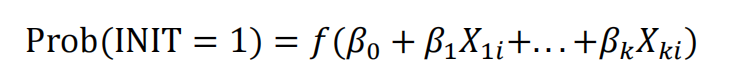
Recall that the dataset “d_div.sas7bdat” already has the firms that initiate dividend payments (the rows with INIT=1) and the firms did not (the rows with INIT=0). The dataset allows us to analyze dividend initiations, since we have data on companies that decided to initiate dividends and companies that decided not to. No surprise here, since the decision to initiate dividend payments is a binary variable, you should use the PROC LOGISTIC to implement your regression model, as

We’ve seen already that it is really bad news when a firm decides to stop paying dividends. So, if the manager decides to start paying dividends, she better be able to anticipate the ability to keep on paying dividends later on. Bottom line is that good financial health should be a requirement before a firm decides to commit to pay dividends. This insight guides the search for the determinants of dividend initiation.

With these in mind let us propose some characteristics that may drive the company’s decision to initiate dividend payments: 实证金融作业代写

· Company size (CSIZE):

companies might need to achieve some level of size before they commit to paying dividends. Company size resembles a bit the definition used in part II. Here company size is defined as the natural logarithm of the market value of equity of the company, measured 24 months. (instead of 12 months used in part II) before the announcement. Market value of equity is defined as MVE=abs(PRC)*SHROUT, where both PRC (stock price). And SHROUT (shares outstanding, measured in thousands of shares) are variables available in the CRSP dataset “msf.sas7bdat” (located in “/wrds/crsp/sasdata/a_stock”). If the announcement date (DCLRDT) happens at month m in year y, collect MVE as of month m of year y – 2.

· PASTROA:

poor-performing firms should definitely not start paying dividends! The proxy for company performance, call it PASTROA, is defined as the average return on assets for the company in the three years preceding the year before the announcement of the dividend initiation. Our definition of PASTPERF resembles the ROA definition in part II. Except for the period of data collection: it is now the average return on assets for the company in the three years between YEAR(DCLRDT) – 4 and YEAR(DCLRDT) -2.

· Recent performance (PASTPERF): 实证金融作业代写

this measure mimics the PERF measure examined in Part II except that the period of data collection precedes one year prior to the announcement date. PASTPERF is defined as the average daily stock return during the calendar period DCLRDT – 365 – 180 and DCLRDT – 365.

· Firm age (AGE):

the younger the firm, the less likely that it will pay dividends (after all, that is the time the firm might be experiencing growth. So it is better to use whatever money is available to fund profitable projects rather than paying the money to investors). The variable AGE is defined as the number of years since the firm went public. The dataset “d_div_first_years.sas7bdat” contains for each firm (identified by its PERMNO) the year the company went public (FIRST_YEAR). You define AGE=YEAR(DCLRDT) – FIRST_YEAR+1.

Prepare and show a summary statistics table of the explanatory variables for the sample with INT=1 vs. the sample with INIT=0. Interpret the numbers.

Then run the logistic regression explaining the likelihood of the company announcing a dividend initiation,

Report the regression results. Discuss the significance of each coefficient, and interpret the effect of each variable on the likelihood that a company announces dividend initiation. The effect should be based on the change in the odds that a firm starts paying dividends. You can play with some specific changes; for example, when examining the effect of changes in ROA. You may examine the effect of having the ROA increase by 0.1—say from 0.1 to 0.2.

Finally, compute the predicted probability of dividend for a company with the following values: MVE=500,000, PASTROA=+0.12, PASTPERF=0.001. And AGE=5 (you can use an Excel worksheet to compute this probability).

Appendix: Some comments and suggestions: 实证金融作业代写

1.

Most if not all of the data analyses here are replications of data analyses implemented in other assignments throughout the course. For example, a very good starting point for the event studies in part I come from the event studies we implemented either in module 4 or in assignment 4. Also, any single control variable described here is some variation of control variables that we used throughout the course.

2.

The same rules on how to generate write-ups for all assignments in the course apply here. In particular, the write-up should not mention SAS or codes. And an appendix should be included with all the codes used in the generation of your outputs. An assignment without a code, or any result that is not supported by a code will not be graded.

3.

The assignment does not demand any output specifically, but it is expected that you produce and show many outputs. For example, if you are going to discuss the results of a regression model, you should generate the output for that regression model. If any result is required for your discussion, you should include it in your write-up. SAS output should be avoided; instead your outputs should be formatted to include only information relevant to the discussion.

4. 实证金融作业代写

Be as precise as you can in your discussion. For example, when examining a relationship between Y and X in a regression framework, make sure you state the hypothesis being tested in an unambiguous way. (e.g., are you testing the regression coefficient based on an one-tailed or two-tailed alternative hypothesis?); then if you need a number to anchor your conclusion (the t statistic), refer to the specific number of your analysis. Then, if needed, examine the magnitude of the effect of X on Y, making sure that you properly describe the units of measurement of the variables involved in the analysis.

5.

The individual assignment deliberately avoids having numbered questions. This way, your write-up is not an attempt to answer questions 1, 2, 3, etc, but to discuss the theme of dividend initiation in a thorough way. Assume that the reader does not have access to this document. So that your write-up should be self-contained in explaining the motivation for the analyses, the methodologies adopted, the results, and the inferences. An example of such a self-contained write-up appears on Canvas, under “Modules”/”Supplementary Material”/”How to Prepare the Write-Up for the Individual Assignment”.

6. 实证金融作业代写

You do not need to be constrained by the control variables (and models) suggested in the assignment. These control variables are a minimum set of variables necessary for the project. If you deem another variable X relevant to, say, explain market reactions to announcements of dividend initiation (part II). You are free to expand the model and include your new variable.

7.

Partial grade is available. If you have problems generating a control variable for your model, ignore it and go ahead with the model without that control variable. Partial grading is not available, though, for a code that does not run. Hence, a strong suggestion is for you to build your model incrementally. For example, in part II, run the simple regression model. If it works, save your code (under a name, say, p1), then try to include one more control variable. If the inclusion is successful, then save the new code (call it p2). Repeat the process with each extra control variable. If you get to a point where the inclusion of an extra variable is unsuccessful, then return the previous version of the code. It is much better to have a partial model that runs than a complete model that does not run.

更多代写：JavaScript代写  托福家考保分  英国代写为什么被发现  美国论文怎么写  dissertation代寫  apa引用格式

合作平台：essay代写 论文代写 写手招聘 英国留学生代写